Matching Algorithms 
A set of rules followed by a computer for finding pairs of matching resources is defined here as a matching algorithm. It can be further categorised as automated or semi-automated depending on whether it requires user assistance or not. Most matching algorithms employed in the Lenticular Lens are semi-automated. This section presents the catalogue of algorithms available in the Lenticular Lens and the standard expected Inputs and Outputs.
The system offers a variety of existing and newly developed algorithms from which the user can choose one or more in order to perform a matching. These algorithms apply for example, to strings, dates or URIs. Here by, we describe the ones currently offered by the system and how they are meant to be used:
-
Exact search
-
Mapping
-
Change / Edit
-
Phonetic
-
Hybrid
Intermediate (exact and mapping)
Soundex Approximation (phonetic and changes/edits)
Approx over Same-Soundex (phonetic and changes/edits)
Word Intersection (in-exact and changes/edits)
TeAM:Text-Approximation-Match (changes/edits and phonetic)
-
Numerical
-
Make use of above methods
1. Discrete Strength
Her we present algorithms for which the resulting strength of a matched pair of resources is assigned the value of 1 as 0 means a match could not be found.
Unknown
A resource used to denote that the method used to generate the current set of links is unknown.
Exact
This method is used to align source and target’s IRIs whenever their respective user selected property values are identical.
In Example-1, the linkset ex:ExactLinkset is generated using the exact method over the predicate rdfs:label. Although only sharing the exact same name, these two entities are clearly not the same.
Example 1: Generating a linkset using the Exact algorithm.
institutes:grid.1019.9
    rdfs:label             "Victoria University" ;
    grid:wikipediaPage      wiki:Victoria_University,_Australia ;
    grid:establishedYear    "1916"^^<http://www.w3.org/2001/XMLSchema#gYear> ;
    gridC:abbreviation>     "VU" ;
    skos:prefLabel          "Victoria University";
   •••

institutes:grid.449929.b
   rdfs:label              "Victoria University" ;
   grid:wikipediaPage       <https://en.wikipedia.org/wiki/Victoria_University_Uganda> ;
   grid:establishedYear     "2011"^^<http://www.w3.org/2001/XMLSchema#gYear> ;
   gridC:abbreviation>      "VUU" ;
   skos:prefLabel           "Victoria University" ;
    •••

ex:ExactLinkset
{
    <<institutes:grid.1019.9   owl:sameAs   institutes:grid.449929.b>>
        ll:hasMatchingStrength  1 .
}
Embedded
The Embedded method extracts an alignment already provided within the source dataset. The extraction relies on the value of the linking property, i.e. property of the source that holds the identifier of the target (IRI of the target). The inconvenience in generating a linkset in such way is that the real mechanism used to create the existing alignment is not explicitly provided by the source dataset.
Example-2 shows a sample of the Grid dataset with embedded links. With such links, Grid connects its instances to external datasets such as Wikidata for example using the link predicate: grid:hasWikidataId illustrated in Example-2 with the linkset graph ex:EmbeddedLinkset.
Example 2: Generating a linkset using the Embedded algorithm.
institutes:grid.1001.0
    foaf:homepage          <http://www.anu.edu.au/> ;
    rdfs:label             "Australian National University" ;
    grid:isni              "0000 0001 2180 7477" ;
    grid:hasWikidataId     wikidata:Q127990 ;
    • • •

institutes:grid.1002.3
    foaf:homepage          <http://www.monash.edu/> ;
    rdfs:label             "Monash University" ;
    grid:isni              "0000 0004 1936 7857" ;
    grid:hasWikidataId     wikidata:Q598841 ;
    • • •

ex:EmbeddedLinkset
{
    <<institutes:grid.1001.0   grid:hasWikidataId   wikidata:Q127990>>
        ll:hasMatchingStrength  1 .

    <<institutes:grid.1002.3   grid:hasWikidataId   wikidata:Q598841>>
        ll:hasMatchingStrength  1 .
}
Intermediate
The method aligns the source and the target’s IRIs via an intermediate database by using properties that potentially present different descriptions of the same entity, such as country name and country code. This is possible by providing an intermediate dataset that binds the two alternative descriptions to the very same identifier.
Example 3.1: Generating a linkset using the Intermediate-Datatse algorithm.
In the example below, it is possible to align the source and target country entities using the properties country and iso-3 via the intermediate dataset because it contains the information described at both, the Source and Target.
dataset:Source-Dataset                       dataset:Intermediate-Dataset
{                                            {
    ex:1  rdfs:label  "Benin" .                 ex:7
    ex:2  rdfs:label  "Cote d'Ivoire" .              ex:name "Cote d'Ivoire" ;
    ex:3  rdfs:label  "Netherlands" .                ex:code "CIV" .
}
                                                ex:8
dataset:Target-Datas                                ex:name "Benin" ;
{                                                   ex:code "BEN" .
    ex:4 ex:iso-3 "CIV" .
    ex:5 ex:iso-3 "NLD" .                       ex:9
    ex:6 ex:iso-3 "BEN" .                           ex:name "Netherlands" ;
}                                                   ex:code "NLD" .
                                             }
# --- ALIGNMENT -----------------------------
#   • If rdfs:label is aligned with ex:name
#   • AND ex:iso-3 is aligned with ex:code,
#   • We then get the following linkset:
# -------------------------------------------
    linkset:Match-Via-Intermediate
    {
        <<ex:1 owl:sameAs ex:6>>
            ll:hasMatchingStrength  1 .

        <<ex:2 owl:sameAs ex:4>>
            ll:hasMatchingStrength  1 .

        <<ex:3 owl:sameAs ex:5>>
            ll:hasMatchingStrength  1 .
    }
Example 3.2: Generating a linkset using the Intermediate-Datatse algorithm.
In this second example, it is also possible to align the source and target datasets using the the authoritative intermediate dataset as it contains information described at both, the Source and Target.
dataset:Source-Dataset                       dataset:Intermediate-Dataset
{                                            {
    ex:10  rdfs:label  "Rembrandt" .             ex:70
    ex:20  rdfs:label  "van Gogh" .                  ex:name "Vincent Willem van Gogh" ;
    ex:30  rdfs:label  "Vermeer" .                   ex:name "Vincent van Gogh" ;
}                                                    ex:name "van Gogh" .
                                                ex:80
dataset:Target-Datas                                ex:name "Rembrandt" ;
{                                                   ex:name "Rembrandt van Rijn" .
    ex:40 schema:name "Rembrandt van Rijn" .
    ex:50 schema:name "Vincent van Gogh" .       ex:90
    ex:60 schema:name "Johannes Vermeer" .           ex:name "Johannes Vermeer" ;
}                                                    ex:name "Vermeer" .
                                             }
# --- ALIGNMENT ------------------------------------
#   • If rdfs:label is aligned with ex:name
#   • AND schema:name is also aligned with ex:name,
#   • we then get the following linkset:
# --------------------------------------------------
    linkset:Match-Via-Intermediate
    {
        <<ex:10 owl:sameAs ex:40>>
            ll:hasMatchingStrength  1 .

        <<ex:20 owl:sameAs ex:50>>
            ll:hasMatchingStrength  1 .

        <<ex:30 owl:sameAs ex:60>>
            ll:hasMatchingStrength  1 .
    }
Soundex
Soundex is a phonetic algorithm for indexing names by sound, as pronounced in English. The goal is for homophones to be encoded to the same representation so that they can be matched despite minor differences in spelling. The algorithm mainly encodes consonants; a vowel will not be encoded unless it is the first letter.
Example 4.a: Generating a linkset using the Soundex algorithm
The examples below shows the encoding of different names. Here, the size parameter indicates a degree of similarity through the length of the respective soundex codes. For example at size=3, Albert and Albertine have the same soundex representation while at size=5 their respective representations differ. In the Lenticular lens, the default size is set to 3.
# -----------------------------
# INPUT          SIZE 3   SIZE 5
# -----------------------------
# A.             A000     A00000
# AL             A400     A40000
# ALI            A400     A40000
# ALBERT         A416     A41630
# ALBERTINE      A416     A41635

ex:128.45
    rdfs:label              "ALBERT" ;
     •••

ex:6852:28
   rdfs:label               "ALBERTINE" ;
    •••

ex:ExactLinkset
{
    <<ex:128.45   owl:sameAs   ex:6852:28>>
        ll:hasMatchingStrength  1.
}
In the Lenticular Lens, Soundex is used as a normaliser in the sense that an edit distance is run over the soundex code version of a name. For example, in the table below, the normalisation/encoding of both Louijs Rocourt and Lowis Ricourt becomes L200 R263 leading to an edit distance of 0 and a relative strength of 1. However, computing the same names using directly an edit distance results in an edit distance of 3 and a relative matching strength of 0. 79.
Example 4.b: Soundex implementation in the Lenticular Lens
--------------
-- Example -- THE USE OF SOUNDEX CODE FOR STRING APPROXIMATION
--------------
The example below shows the implementation of Soundex Distance
in the Lenticular Lens and how it compares with Edit Distance
over the original names (no soundex-based normalisation).

------------------------------------------------------------------------------------------------------------------------------------------------------
Source                      Target                     E. Dist  Rel. distance  Source soundex       Target  soundex       Code E. Dist  Code Rel. Dist
------------------------------------------------------------------------------------------------------------------------------------------------------
Jasper Cornelisz. Lodder    Jaspar Cornelisz Lodder          2           0.92  J216 C654 L360       J216 C654 L360                   0             1.0
Barent Teunis               Barent Teunisz gen. Drent       12           0.52  B653 T520            B653 T520 G500 D653             10            0.47
Louijs Rocourt              Louys Rocourt                    2           0.86  L200 R263            L200 R263                        0             1.0
Louijs Rocourt              Lowis Ricourt                    3           0.79  L200 R263            L200 R263                        0             1.0
Louys Rocourt               Lowis Ricourt                    3           0.77  L200 R263            L200 R263                        0             1.0
Cornelis Dircksz. Clapmus   Cornelis Clapmuts               10            0.6  C654 D620 C415       C654 C415                        5            0.64
Geertruydt van den Breemde  Geertruijd van den Bremde        4           0.85  G636 V500 D500 B653  G636 V500 D500 B653
See approximation over same soundex and approximation over soundex encoding for more information on how the algorithm is implemented in the Lenticular Lens.
Metaphone
Designed by Lawrence Philips in 1990, Metaphone is a phonetic algorithm for a more accurate encoding of words by sound (as compared to SOUNDEX) as pronounced in English. In this algorithm as with SOUNDEX, similar-sounding words should share the same encoding key which is an approximate phonetic representation of the original word.
For more accuracy, consider the use of Double Metaphone as it is an improvement of the Original Metaphone. In turn, for an even better improved accuracy, consider the use of Metaphone 3.
See approximation over same soundex and approximation over soundex encoding for more information on how the algorithm is implemented in the Lenticular Lens.
Double Metaphone
Double Metaphone is a third generation phonetic algorithm improvement after Soundex and Metaphone for an accurate encoding of words by sound as pronounced in English. For more accuracy, consider the use of METAPHONE 3 as it is an improvement of the Double Metaphone algorithm.
It is called “Double” because it can return both a primary and a secondary code for a string; this accounts for some ambiguous cases as well as for multiple variants of surnames with common ancestry. For example, encoding the name “Smith” yields a primary code of SM0 and a secondary code of XMT, while the name “Schmidt” yields a primary code of XMT and a secondary code of SMT—both have XMT in common.
Double Metaphone tries to account for myriad irregularities in English of Slavic, Germanic, Celtic, Greek, French, Italian, Spanish, Chinese, and other origin. Thus it uses a much more complex ruleset for coding than its predecessor; for example, it tests for approximately 100 different contexts of the use of the letter C alone.
See [https://en.wikipedia.org/wiki/Metaphone] for mor information. See also approximation over same soundex and approximation over soundex encoding for more information on how the algorithm is implemented in the Lenticular Lens.
NYIIS
TODO
Example 7:
Numbers
The method is used to align the source and the target IRIs whenever the delta difference between values (number/date) of the user selected properties is within a preset delta-threshold.
Example 8
For example, if two entities have been aligned based on the similarity of their names but an extra check is to be investigated based on their respective year of birth, setting the delta-threshold to 1 year will ensure that the birth dates assigned to the two entities are no more than one year apart.
Time Delta
This function allows for finding co-referent entities on the basis of a minimum time difference between the times reported by the source and the target entities. For example, if the value zero is assigned to the time difference parameter, then, for a matched to be found, the time of the target and the one of the source are to be the exact same times. While accounting for margins of error, one may consider a pair of entities to be co-referent if the real entities are born lambda days, months or years apart among other-things (similar name, place..).
Time Delta before, After or Between. Other ways of using time delta are also possible. Because Time Delta has no direction or sign (+ or -), it is not possible to require that the time documented at the source entity occurs before or after the one reported by the target’s event. With the before / After options, this is possible. Using the Between option, we make it possible for the user to define the time interval in which both the source and target reported times can be viewed as acceptable.
Example 9:
Same Year Month
This option is used to align source and target’s IRIs whenever an exact match of the year or year and month is observed between source and target’s input dates.
2. Continuous Strength
Her we present algorithms for which the resulting strength of a matched pair of resources is in the range ]0, 1] where 0 means a match could not be found while 1 means a perfect match is found.
Jaro
This method is used to align source and target’s IRIs whenever the similarity score of their respective user selected property values are above a given threshold in the range ]0, 1].
Jaro distance is a measure of similarity between two strings. The higher the Jaro distance for two strings is, the more similar the strings are. The score is normalised such that 0 equates to no similarity and 1 is an exact match.
Given two strings s1 and s2,
- Find common characters xi from s1 and yj from s2 such that xi = yj where xi and yj are not more than d characters aways from each other and where the acceptable matching distance d is half the longest input string as expressed in the formula:
-
Let c be number of common characters shared by s1 and s2.
-
From the resulting common characters in s1 and s2, let t be the number of transposition which is the number of characters that do not share the same position.
- Compute the strength using the formula:
Example 10: Jaro results
SOURCE                : |s| = |source| = 6
TARGET                : |t| = |target| = 6
MATCHING DISTANCE     : d = max(6, 6) = 3
COMMON CHARACTERS     : m = |re| = |re| = 2
TRANSPOSITIONS        : t = 0
STRENGTH              : s = 1/3 * ( 2/6 + 2/6 + (2 - 0/2)/2) = 0.55556


SOURCE                : |s| = |jono| = 4
TARGET                : |t| = |ojhono| = 6
MATCHING DISTANCE     : d = max(4, 6) = 3
COMMON CHARACTERS     : m = |jono| = |ojon| = 4
TRANSPOSITIONS        : t = 4
STRENGTH              : s = 1/3 * ( 4/4 + 4/6 + (4 - 4/2)/4) = 0.72222


SOURCE                : |s| = |DUANE| = 5
TARGET                : |t| = |DWAYNE| = 6
MATCHING DISTANCE     : d = max(5, 6) = 3
COMMON CHARACTERS     : m = |DANE| = |DANE| = 4
TRANSPOSITIONS        : t = 0
STRENGTH              : s = 1/3 * ( 4/5 + 4/6 + (4 - 0/2)/4) = 0.82222


SOURCE                : |s| = |DIXON| = 5
TARGET                : |t| = |DICKSONX| = 8
MATCHING DISTANCE     : d = max(5, 8) = 4
COMMON CHARACTERS     : m = |DION| = |DION| = 4
TRANSPOSITIONS        : t = 0
STRENGTH              : s = 1/3 * ( 4/5 + 4/8 + (4 - 0/2)/4) = 0.76667


SOURCE                : |s| = |JELLYFISH| = 9
TARGET                : |t| = |SMELLYFISH| = 10
MATCHING DISTANCE     : d = max(9, 10) = 5
COMMON CHARACTERS     : m = |ELLYFISH| = |ELLYFISH| = 8
TRANSPOSITIONS        : t = 0
STRENGTH              : s = 1/3 * ( 8/9 + 8/10 + (8 - 0/2)/8) = 0.8963
Jaro-Winkler
Given two strings s1 and s2, the Winkler similarity equation boosts up the Jaro algorithm’s result dj by increasing it whenever the compared strings share a prefix of a maximum of four characters. In this shared prefix scenario, the boost is computed as:
where Pl is the length of the set of shared prefix and Pw is a user dependent scaling factor for how much the score is adjusted upwards for having common prefixes. Because four is the maximum number of shared prefix to consider, the user’s choice of Pw lies between 0 and ¼. Setting Pw to ¼ implies a similarity of always 1 whenever the strings share the maximum of 4 prefixes, no matter the real dissimilarity between the strings.
The Jaro-Winkler is computed as:
Example 11: Jaro vs Jaro-Winkler
jaro("alexander", "alexandrine") = 0.90236
jaro_winkler("alexander", "alexandrine", weight=0.1) = 0.94141
Levenshtein
This method is used to align source and target’s IRIs whenever the similarity score of their respective user selected property values are above a given Levenshtein Distance threshold.
Levenshtein (a.k.a. Edit Distance) is a way of quantifying how dissimilar two strings (e.g., words) are to one another by counting the minimum number of operations ε (removal, insertion, or substitution of a character in the string) required to transform one string into the other. For example, the Levenshtein distance between “kitten” and “sitting” is ε = 3 as it requires two substitutions (“s” for “k” and “i” for “e”) and one insertion of “g” at the end.
Normalisation Ω: In the Lenticular Lens, the similarity score Ω of a matching pair of resources is quantified in the interval [0, 1]. For this, the dissimilarity score ε expressing the minimum number of operations to perform for two strings to be the same is normalised as Ω based on the length of the longest string. The dissimilarity score ε = 3 between ”kitten” and “sitting” is then normalised to a similarity score Ω = 1 - 3 / 7 = 0.57.
Minimum threshold φ: Using this algorithm, a minimum threshold valueφ must be set in the interval [0,1], such that finding any matched pairs of IRIs based on the similarity of their respective property values depends on whether or not the computed Ω is equal or above φ. A threshold φ = 1 equates an exact match. In our previous example, if a minimum threshold of φ = 0.7 is set, “kitten” and “sitting” will not be matched. In short, φ is the user defined threshold when the similarity score Ω is selected for accepting or rejecting a match.
Maximum character error threshold 𝛿: In case the original edit distance score ε (minimum number of operations score) is preferred, the number of character errors 𝛿 of choice is used instead as threshold for deciding whether a match is accepted or rejected. However, for consistency purposes, the corresponding normalisation value Ω is still computed for the minimum number of operations score computed ε. For instance, in our previous example, if a maximum characters errors is set to 𝛿 = 3, “kitten” and “sitting” will be matched but the computed strength will be Ω = 0.57 and not ε = 3 as is it only serves the purpose of decision maker. In short, 𝛿 is the user defined threshold when the dissimilarity score ε is selected for accepting or rejecting a match.
Example 12: The Levenshtein options
1. l_dist(Rembrand van Rijn, Rembrandt Harmensz van Rijn) = 10
2. Normalised_l_dist (Rembrand van Rijn, Rembrandt Harmensz van Rijn) = 0.63
>>> If φ (Minimum threshold) = 0.7
>>> then [Rembrand van Rijn] owl:sameAs [Rembrandt Harmensz van Rijn]
>>> is rejected
>>> because Ω = 0.63 < φ.
>>> If δ (Maximum character error threshold) = 5
>>> then [Rembrand van Rijn] and [Rembrandt Harmensz van Rijn] is rejected
>>> because ε = 10 > δ.
Trigram
Trigrams are a special case of the n-gram, where n is 3. It is a contiguous sequence of three items from a given sample. To be more concrete, In the case of string similarity, where an application of name is a sample and a character is an item, we obtain a sequence of 4 trigrams { mar | art | rth | tha } from the sample martha. If we now consider a word as an item in the sample “the quick red fox jumps over the lazy brown dog”, we then obtain a sequence of 8 word-level trigrams { the quick red | quick red fox | red fox jumps | fox jumps over | jumps over the | over the lazy | the lazy brown | lazy brown dog }.
N-grams can be used for approximate matching by comparing two trigram sequences using metrics such as cosine distance, z-scores or g-test. In such a use case, the method is used to align the source and the target IRIs whenever the computed similarity strength is equal to or above a user-predefine value.
Soundex Approximation
This option is performed in two phases to align the source and the target IRIs. First, the string values of the user selected properties are encoded (converted to a soundex code). Then a user selected matcher (Levenshtein, Jaro, jaro-Winkler…) is run over the encoded string (Soundex code).
Example 13: Links found using soundex
In the example below, given ex:E1 and ex:E2, the matching strength using Edit Distance is 1 - ⅛ = 0.875. When directly performing an Edit distance match or a Soundex, we respectively get 0.625 and 0 as strengths.
# -------------------------------
# INPUT          SIZE 3   SIZE 4
# -------------------------------
# Carretta       C630     C6300
# Kareta         K630     K6300

ex:E1  rdfs:label  "Carretta" .
ex:E2  rdfs:label  "Kareta" .

ex:ExactLinkset
{
    <<ex:E1   skos:closeMatch   <ex:E2>> ll:hasMatchingStrength  0.875.
}
Approx over Same-Soundex
In the Lenticular Lens, Soundex can also be used as a first filtering step (string normalisation). This means that first we select all pairs sharing the same Soundex code. Then, for each of these pairs an extra string sequence matching algorithm such as (Levenshtein, Jaro, Jaro-Winkler…) is applied to the original pair of matched strings (not the Soundex codes) to determine the strength of the match in the interval ]0, 1].
Example 14: Generating a linkset using the Soundex algorithm.
In the table below, the normalisation of both Louijs Rocourt and Lowis Ricourt becomes L200 R263 leading to an edit distance of 0 and a relative strength of 1. However, computing the same names using directly an edit distance results in an edit distance of 3 and a relative matching strength of 0.79.
The example below shows the implementation of Soundex Distance
in the Lenticular Lens and how it compares with Edit Distance
over the original names (no soundex-based normalisation).

------------------------------------------------------------------------------------------------------------------------------------------------------
Source                      Target                     E. Dist  Rel. distance  Source soundex       Target  soundex       Code E. Dist  Code Rel. Dist
------------------------------------------------------------------------------------------------------------------------------------------------------
Jasper Cornelisz. Lodder    Jaspar Cornelisz Lodder          2           0.92  J216 C654 L360       J216 C654 L360                   0             1.0
Barent Teunis               Barent Teunisz gen. Drent       12           0.52  B653 T520            B653 T520 G500 D653             10            0.47
Louijs Rocourt              Louys Rocourt                    2           0.86  L200 R263            L200 R263                        0             1.0
Louijs Rocourt              Lowis Ricourt                    3           0.79  L200 R263            L200 R263                        0             1.0
Louys Rocourt               Lowis Ricourt                    3           0.77  L200 R263            L200 R263                        0             1.0
Cornelis Dircksz. Clapmus   Cornelis Clapmuts               10            0.6  C654 D620 C415       C654 C415                        5            0.64
Geertruydt van den Breemde  Geertruijd van den Bremde        4           0.85  G636 V500 D500 B653  G636 V500 D500 B653              0             1.0
Bloothooft
This approximation method is specifically tailored for accessing the similarity between a pair of IRIs for which the user selected property values are Dutch names. The algorithm basically normalises the given names by removing or replacing specific characters…. The resulting normalised names are then pairwise compared using the Approximated Levenshtein Distance (see the description of Approximated Levenshtein Distance).
Example 15:
Word Intersection
This approximation method is originally designed to find a subset of words within a larger text. However, it could also be used for any pair of strings regardless of the strings sizes. Several options are available:
- Whether or not the order in which the words are found is important.
- Whether or not the computed strength of each word should be approximated or identical.
- Whether or not abbreviation should be detected.
- Whether the default stopping character should be used, not used or modified.
- A threshold on the number of words not approximated/identical.
- An overall threshold for accepting or rejecting a match.
Example 16: Expectation
For example, it can be used for aligning - [Rembrand van Rijn] and [van Rijn Rembrandt] - [Herdoopers anslagh op Amsterdam] and [Herdoopers anslagh op Amsterdam. Den x. may: 1535. Treur-spel.] regardless of the words’ order.
Example 1
With argument APPROX set to True, similarity can be found between Rembrand and Rembrandt (MODE-1). However, this is not possible in the inverse scenario (MODE-2). Furthermore, when the order is of no importance (MODE-1) the sequence in which the intersection of words appears is of no importance.
       SMALL : Rembrand (van) Rijn
         BIG : Rembrandt Harmensz. van Rijn

      MODE-1 : APPROX = True and ORDER = False
       FOUND : ['rijn', 'rembrandt']
    STRENGTH : 0.97059

      MODE-2 : APPROX  = False and ORDER = True and
       FOUND : []
    STRENGTH : 0.0
Example 2
Because the match is performed over exact occurrences (APPROX = False) and the sequence in which the matched words appear in the text is of importance (ORDER = True), elvervelt is the only intersection found in MODE-2 and thereby bringing the similarity strength to 0.333.
       SMALL : Elvervelt, Henrik van
         BIG : Henrik van Elvervelt

      MODE-1 : APPROX = True and ORDER = False
       FOUND : ['elvervelt', 'henrik', 'van']
    STRENGTH : 1.0

      MODE-2 : APPROX = False and ORDER = True and
       FOUND : ['elvervelt']
    STRENGTH : 0.333
Example 3
In here all intersected words appear in the same sequence and without mismatch.
       SMALL : Herdoopers anslagh op Amsterdam
         BIG : Herdoopers anslagh op Amsterdam. Den x. may: 1535. Treur-spel.

      MODE-1 : APPROX = True and ORDER = False
       FOUND : ['herdoopers', 'anslagh', 'op', 'amsterdam']
    STRENGTH : 1.0

      MODE-2 : APPROX = False and ORDER = True and
       FOUND : ['herdoopers', 'anslagh', 'op', 'amsterdam']
    STRENGTH : 1.0
List Intersection
This method is better suited for matching events. It helps establishing a relationship between the source and target entities whenever a list of entities from the source dataset intersects another list of entities stemmed from the target dataset.
For illustration, suppose that we have the two events in Example-17. (1) Event one, defined by the source event-entities, documents event-entities that lists entities representing persons about to get married. This event is the Intended-Marriage event. (2) Event two is the Marriage event. It lists (i) entities representing persons that got married and (ii) the guests who attended the event.
Now that the two events are defined, let us imagine that we would like to find out which of the Intended-Marriage couple fulfilled its will to get married. For this to be true, we assume that a couple with the wish to be wed should end-up being present at a Marriage event, hopefully their own marriage. This means that, for a match to occur, a minimum of two elements from a list from the source must also belong to a list from the target. In other words, a match is to be generated whenever 100% (all) of the elements in a source’s lists intersects a target’s list.
In this method, two thresholds are to be defined.
-
The first threshold or similarity-threshold imposes a minimum accepted similarity score (generally in ]0, 1]) when elements stemmed from different lists are compared. Passing this threshold is interpreted as the occurrence of an intersection between elements of two lists.
-
The second threshold, the intersection-threshold expressed in quantity or percentage, denotes the minimum number of intersections that must occur for a link to be created.
In practice, looking at Example-17, only events ex: intended-1 and ex:married-2 are a match as the pairs (Catharina Reminck , Catharina Remink) and (Mr. Jean van de Melie, J. van de Melie) are respectively similar with a score of 0.94 and 0.82.
Example 17: List Intersection
A source dataset documenting events as lists of couple with the intention of getting married and a target dataset with list of people at a wedding ceremony. Each of these latter lists is expected to includes the wed couple.
---------------------------------------------------------------------------------------------
Source Dataset                              Target Dataset
---------------------------------------------------------------------------------------------

ex:intended-1                               ex:ceremony-1
    ex:wife     "Catharina Reminck" ;            ex:participant  "Pieter Jas" ;
    ex:husband  "Mr. Jean van de Melie" .        ex:participant  "Jacob Poppen" ;
                                                 ex:participant  "Gillis Graafland" ;
ex:intended-2                                    ex:participant  "Jacob Fransz. de Witt" ;
    ex:wife     "Eva Oostrom"  ;                 ex:participant  "Elisabeth van Daaken" ;
    ex:husband  "Pieter de Vriest" .             ex:participant  "Catharina Berewouts" ;
                                                 ex:participant  "Aafje Hendricx" ;
ex:intended-3                                    ex:participant  "Anthony van Paembergh" ;
    ex:wife     "Eva Oostrom" ;                  ex:participant  "Eva van Toorn" ;
     ex:husband  "Wiggert van Wesick" .          ex:participant  "Maria Bor" .

                                            ex:married-2
                                                ex:participant  "J. van de Melie" ,
                                                    "Bernardus van Vijven" .
                                                    "Margrita Schrik" ,
                                                    "Johannes de Bruijn" ,
                                                    "Maria Gosina Demol" ,
                                                    "Agneta Swartepaart",
                                                    "Hendrik de Lange" ,
                                                    "Catharina Remink" .

ex:intended-4                               ex:ceremony-2
    ex:wife      "Catharina Elisabet" ;          ex:participant "Pieter Robidé" ,
    ex:husband   "Pieter Robidé" .                  "Jacob Fredrik" ,
                                                    "Petronella Hobbe" ,                                                         "Catharina Maria Boom" ,
                                                    "Pieter Robie" ,
                                                    "Fredrik Arentse" .
With a Similarity-threshold set to 0.8 and an Intersection-threshold set to 2 or 100%, only events ex:intended-1 and ex:married-2 are a match as the pairs (Catharina Reminck , Catharina Remink) and (Mr. Jean van de Melie, J. van de Melie) are respectively similar with similarity scores of 0.94 and 0.82.
TeAM
The TeAM (Text Approximation Match) method allows for the approximation of the relevance of a document to a query. Such approximation can be done using lexical similarity (word level similarity), semantic similarity or hybrid similarities. In this method, the focus is rather on the lexical similarity. Although tailored to text, it has been adapted to also be applicable to name-based similarity. We now provide an overview of the motivation context supporting the design and implementation of the algorithm.
The Amsterdam’s city archives (SAA) possesses physical handwritten inventories records where a record may be for example an inventory of goods (paintings, prints, sculpture, furniture, porcelain, etc.) owned by an Amsterdamer and mentioned in a last will. Interested in documenting the ownership of paintings from the 17th century, the Yale University Professor John Michael Montias compiled a database by transcribing 1280 physical handwritten inventories (scattered in the Netherlands) of goods. Now that a number of these physical inventories have been digitised using handwriting recognition, one of the goals of the Golden Agent project is to identify Montias’ transcriptions of painting selections within the digitised inventories. This problem can be generically reformulated as, given a source-segment database (e.g. Montias DB) and a target-segment database (e.g. SAA), find the best similar target segment for each source segment.
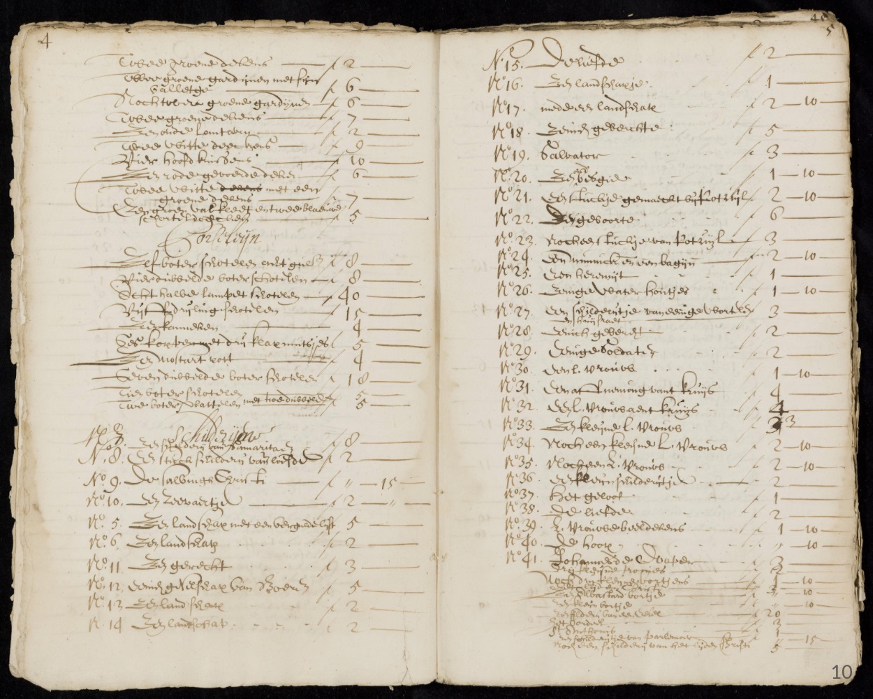 Fig 4.9: Digitisation of inventory documents available at the Amsterdam’s city archives.